Local Spatial Analysis (LSA)
This is an easy-to-use and conceptually-simple adaptive EEG filter, to be used for highlighting local components which are masked by large widespread activity.
At each timepoint, it attempts to regress out the trial-by-trial variability of widespread stimulus-evoked neural activity. In this way, it can uncover underlying local components if certain assumptions are met.
LSA is available as an EEGLAB plugin here:
[Download EEGlab plugin]
[Plugin Tutorial]
This method has been published as Bufacchi et al (2021).
|
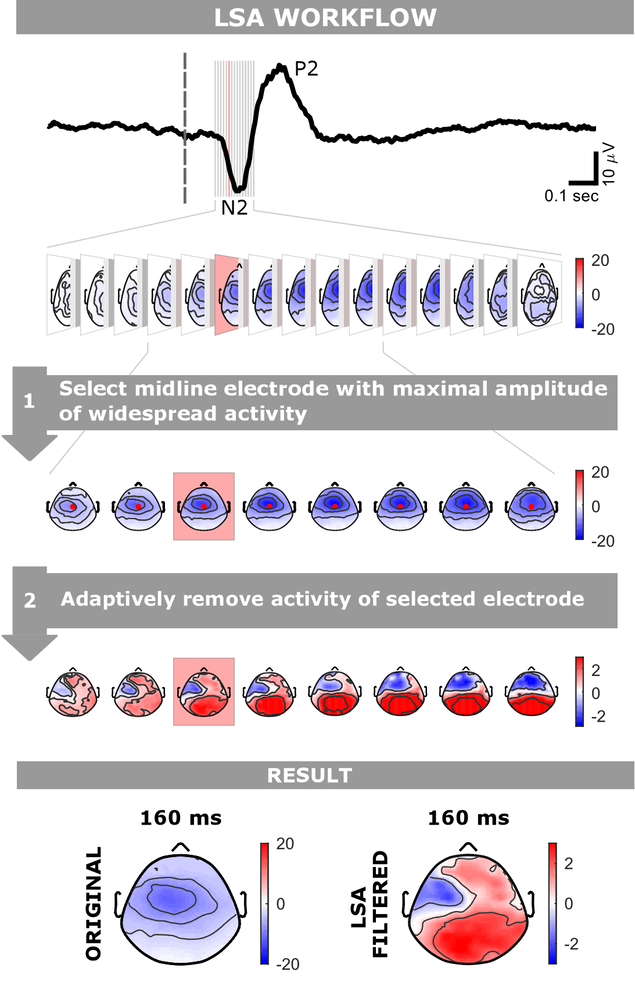
Example procedure for filtering EEG data using LSA.
The filter is applied to real laser-evoked ERPs. Step 1: First, the electrode at which the widespread N2 component is maximal in amplitude is identified in the grand average scalpmap series. In this example, the electrode is Cz. Second, the time interval including the widespread signal (i.e. the interval during which most electrodes have the same polarity) is selected. In this example, the interval is 130-220 ms. Step 2: LSA exploits the different trial-by-trial variability of the local vs the widespread component, and thereby removes the activity from the identified electrode (Cz) from all other electrodes. This is done separately for each subject and time point. The last row shows the comparison of the topography at the same time point (in this example, 160 ms) before and after filtering with LSA. Color bars represent voltage (µV). |
|
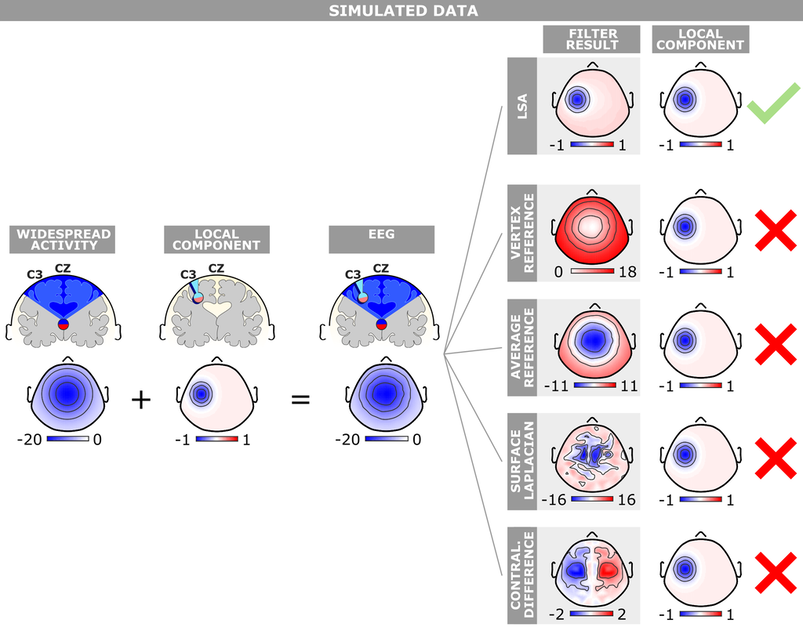
Example performance of LSA on simulated ERP data containing a central widespread component and a lateralised local component. Left panel: EEG topographies were generated as a widespread component at Cz plus a local negative component at C3. Right panel: By exploiting the information contained in the trial-by-trial variability of the simulated data, LSA returns a scalp topography virtually identical to that of the original local component. Commonly-used stationary filters (Vertex Reference, Average Reference, Surface Laplacian) failed to highlight the local component. Only the Contralateral Difference returned a negativity in the left hemisphere, although it also created a spurious positivity in the contralateral hemisphere. Color bars represent voltage (µV).
|
A quick video tutorial for using the plugin is available here: